Disasters in the mines
The package boot contains the dates of coal mining disasters from 1851 to 1962.1
library(boot)     #for coal data
data(coal)
year <- floor(coal)
y <- table(year)
plot(y)  #a very simple time series plot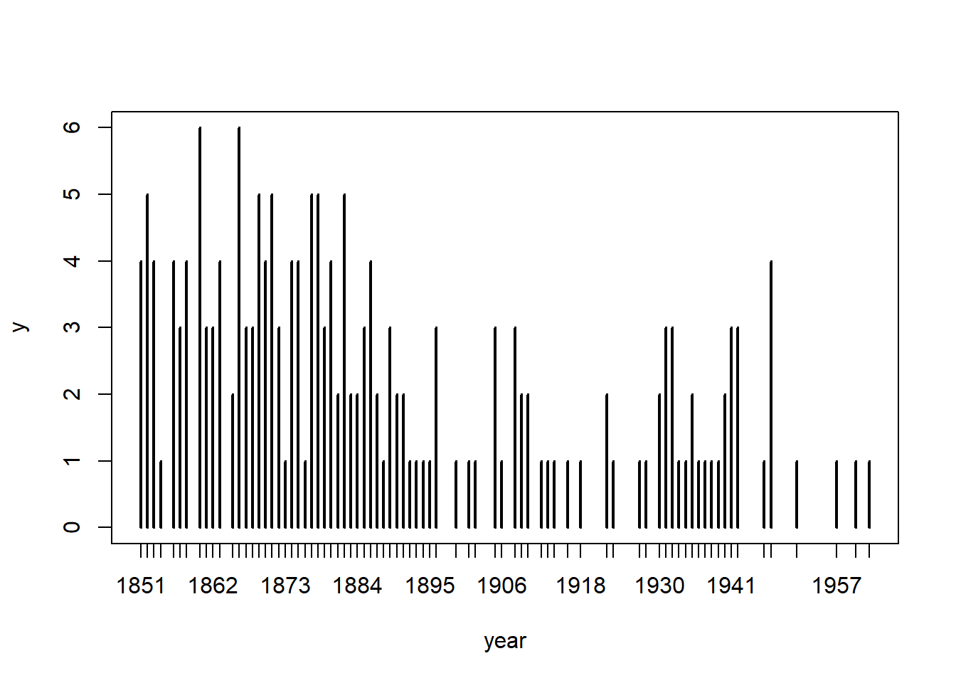
y## year
## 1851 1852 1853 1854 1856 1857 1858 1860 1861 1862 1863 1865 1866 1867 1868 1869
## 4 5 4 1 4 3 4 6 3 3 4 2 6 3 3 5
## 1870 1871 1872 1873 1874 1875 1876 1877 1878 1879 1880 1881 1882 1883 1884 1885
## 4 5 3 1 4 4 1 5 5 3 4 2 5 2 2 3
## 1886 1887 1888 1889 1890 1891 1892 1893 1894 1895 1896 1899 1901 1902 1905 1906
## 4 2 1 3 2 2 1 1 1 1 3 1 1 1 3 1
## 1908 1909 1910 1912 1913 1914 1916 1918 1922 1923 1927 1928 1930 1931 1932 1933
## 3 2 2 1 1 1 1 1 2 1 1 1 2 3 3 1
## 1934 1935 1936 1937 1938 1939 1940 1941 1942 1946 1947 1951 1957 1960 1962
## 1 2 1 1 1 1 2 3 3 1 4 1 1 1 1The plot shows a marked difference in the frequency of disasters before the 1890’s and after. We use the [[]] operator to convert the data frame into a simple numerical series then take the floor of the series to isolate the integer years. The tabulate() function will count the number of disasters for each year. We will only need the tail of the tabulation from 1851 onward.
y <- floor(coal[[1]])
y <- tabulate(y)
y <- y[1851:length(y)]
n <- length(y)
n
## [1] 112A model emerges from the depths
The frequency of disasters, and other rare events, is often modelled with the Poisson distribution. We let \(Y_i\) be the number of disasters in year \(i\), for \(i=i,\cdots,n\), with $n = $ 112. The switch point \(k\) will indicate the index of the year when the Poisson distribution intensity switches from \(\mu\) to \(\lambda\).
\[ \begin{align} Y_i &\sim \operatorname{Poisson}(\mu). &i=1, \ldots, k, \\ Y_i &\sim \operatorname{Poisson}(\lambda). &i=k+1, \ldots, n. \\ \end{align} \]
We might expect the switch point k to be a simple unknown following an uninformative uniform distribution. We could expect the \(mu\) and \(\lambda\) free parameters to follow independent Gamma distributions following actuarial practice.
\[ \begin{align} k &\sim \operatorname{Uniform}(1,\ldots,n), \\ \mu &\sim \operatorname{Gamma}(0.5, b_1), \\ \lambda &\sim \operatorname{Gamma}(0.5, b_2). \end{align} \] The Gamma shapes are just 0.50, but we need to introduce the \(b_1\) and \(b_2\) rates to ensure that the rates are positive multiples of chi-squared distributions. After all, the right-skewed chi-squared distribution seems favored by variables that claim to model volatility. These parameters are fully conditioned on each other on just about everything else in this specification.
\[ \begin{align} b_1 \mid Y, \mu, \lambda, b_2, k &\sim \operatorname{Gamma}(0.5, \mu+1) \\ b_1 \mid Y, \mu, \lambda, b_1, k &\sim \operatorname{Gamma}(0.5,\lambda+1) \end{align} \]
The plus 1 rates in the Gamma priors will iterate from an initial estimate of \(\mu\) or \(\lambda\) by adding 1 on each iteration. After all these are all average counts of disasters per year. All of this conditioning effectively creates cross-distribution constraints. In fact, we need to re-express the \(\mu\) and \(\lambda\) priors conditionally as well in order to allow the counting of the ways in which the switch point \(k\) might evolve when we confront data \(Y_i\). We carry out this confrontation by summing disasters from year 1 to (as yet not known) \(k\) so that
\[ S_k = \Sigma_1^k Y_i \] and from \(k+1\) to \(n\) as
\[ \Sigma_{k+1}^n Y_i = \Sigma_{1}^n Y_i - S_k = S_n -S_k \]
\[ \begin{align} \mu \mid Y, \lambda, b_1, b_2, k &\sim \operatorname{Gamma}(0.5 + S_k, b_1 + k) \\ \lambda \mid Y, \mu, b_1, b_2, k &\sim \operatorname{Gamma}(0.5 + (S_n-S_k), b_2 + n-k) \end{align} \]
We still need a likelihood function \(L\) to carry out the rest of the routine. \(L\) is the probability that the hypothesized parameter \(k\) is consistent with the data as well as the expectations about the parameters that criss-cross this problem. The two Poisson distributions that we began our analysis with have together an implicit switch point. However, we need a data likelihood that is explicitly sensitive to the switching point. This point acts like a threshold in dividing the sample into two regimes. A distribution with this property is the Pareto distribution. We will use this likelihood instead of the two Poissons we started with.
\[ L(Y \mid \mu, \lambda, k) = e^{(\lambda - \mu)} \left( \frac{\mu}{\lambda} \right)^{S_k} \] The first term is the probability we expect for the difference in the two switching regimes delimited by the sum \(S_k\). The second term is the Pareto power distribution with the probability that we see the data given the frequency of one regime relative to the other. Each term embeds the prior distributions of the hypothesized parameters. Finally we compute a normalized likelihood to generate the posterior distribution \(f\) of \(k\).
\[ f(k \mid Y, \mu, \lambda, b_1, b_2) = \frac{L(Y \mid \mu, \lambda, k)}{\Sigma_j^n L(Y \mid \mu, \lambda, j)} \]
Gibbs sampler for the coal mining change point
The Gibbs sampler, as described by Geman and Geman (1984), attempts to sample each free parameter one at at time using the previous parameters as grist for its mill.
First we specify the setup.
# initialize
n <- length(y)    #length of the data
m <- 1000         #length of the chain
mu <- lambda <- k <- numeric(m)
L <- numeric(n)
k[1] <- sample(1:n, 1)
mu[1] <- 1
lambda[1] <- 1
b1 <- 1
b2 <- 1
Next, we run the sampler.
for (i in 2:m) {
        kt <- k[i-1]  # this is Gibbs: work back from the value at i to the value at i-1
                      # then go step by step into the layers of each distribution
                      # the ensemble of layers is the Gibbs lattice
        # generate mu
        r <- .5 + sum(y[1:kt])
        mu[i] <- rgamma(1, shape = r, rate = kt + b1)
        #generate lambda
        if (kt + 1 > n) r <- .5 + sum(y) else
            r <- .5 + sum(y[(kt+1):n])
        lambda[i] <- rgamma(1, shape = r, rate = n - kt + b2)
        # generate new b1 and b2 for the next iteration
        # this is where the averages get incremented
        b1 <- rgamma(1, shape = .5, rate = mu[i]+1)
        b2 <- rgamma(1, shape = .5, rate = lambda[i]+1)
        # generate a sampled likelihood and normalize it
        for (j in 1:n) {
            L[j] <- exp((lambda[i] - mu[i]) * j) *
                          (mu[i] / lambda[i])^sum(y[1:j])
            }
        L <- L / sum(L)
        # generate a single k at iteration i from the discrete distribution L on 1:n
        k[i] <- sample(1:n, prob=L, size=1)
    }
Let’s see some results. First we strip out the first 200 burn-in runs. Then we calculate arithmetic means of \(k\), \(\mu\) and \(\lambda\).
library(tidybayes)
b <- 201
j <- k[b:m]
mean(k[b:m])
## [1] 39.9275mean(lambda[b:m])## [1] 0.9207605mean(mu[b:m])## [1] 3.128555mode_hdci(k)## y ymin ymax .width .point .interval
## 1 41 35 45 0.95 mode hdcihist(k)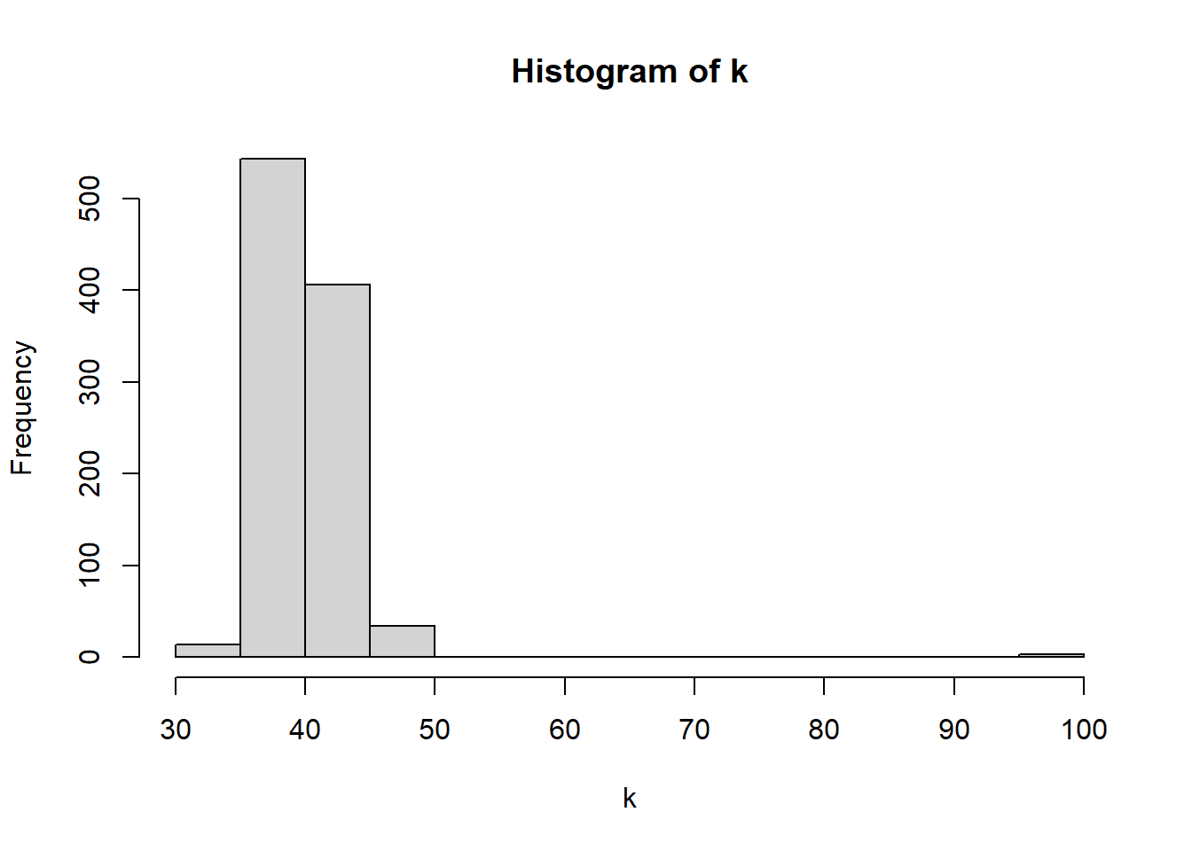
The stochastic switch point occurs at year 40 or year 1890. Prior to this year, on average there were 3 disasters per year. After this year there was 1 disaster per year. There is a 95% probability that the model is compatible with the data between the years 1886 through 1896.
What happened around 1890?
In 1891, Congress passed the first federal statute governing mine safety. The 1891 law applied only to mines in U.S. territories, and, among other things, established minimum ventilation requirements at underground coal mines and prohibited operators from employing children under 12 years of age. The model accurately identifies the stochastic switch point as the year before this legislation.
From 1900 to 1910, the number of coal mine fatalities exceeded 2,000 annually. Congress established the Bureau of Mines as an agency in the Department of the Interior. The Bureau was charged with the responsibility to conduct research and to reduce accidents in the coal mining industry. Inspection authority was granted in 1941.
The Federal Coal Mine Safety Act of 1952 provided for annual inspections and gave the Bureau of Mines limited enforcement authority, including power to issue violation notices and imminent danger withdrawal orders. The 1952 Act also authorized the assessment of civil penalties against mine operators for noncompliance with withdrawal orders or for refusing to give inspectors access to mine property.
Session Info
sessionInfo()## R version 4.0.2 (2020-06-22)
## Platform: x86_64-w64-mingw32/x64 (64-bit)
## Running under: Windows 10 x64 (build 19041)
##
## Matrix products: default
##
## locale:
## [1] LC_COLLATE=English_United States.1252
## [2] LC_CTYPE=English_United States.1252
## [3] LC_MONETARY=English_United States.1252
## [4] LC_NUMERIC=C
## [5] LC_TIME=English_United States.1252
##
## attached base packages:
## [1] parallel stats graphics grDevices utils datasets methods
## [8] base
##
## other attached packages:
## [1] tidybayes_2.1.1 boot_1.3-25 rethinking_2.13
## [4] rstan_2.21.2 StanHeaders_2.21.0-6 forcats_0.5.0
## [7] stringr_1.4.0 dplyr_1.0.1 purrr_0.3.4
## [10] readr_1.3.1 tidyr_1.1.1 tibble_3.0.3
## [13] ggplot2_3.3.2 tidyverse_1.3.0
##
## loaded via a namespace (and not attached):
## [1] matrixStats_0.56.0 fs_1.5.0 lubridate_1.7.9
## [4] httr_1.4.2 tools_4.0.2 backports_1.1.7
## [7] R6_2.4.1 DBI_1.1.0 colorspace_1.4-1
## [10] ggdist_2.2.0 withr_2.2.0 tidyselect_1.1.0
## [13] gridExtra_2.3 prettyunits_1.1.1 processx_3.4.4
## [16] curl_4.3 compiler_4.0.2 cli_2.0.2
## [19] rvest_0.3.6 HDInterval_0.2.2 arrayhelpers_1.1-0
## [22] xml2_1.3.2 bookdown_0.20 scales_1.1.1
## [25] mvtnorm_1.1-1 callr_3.5.1 digest_0.6.25
## [28] rmarkdown_2.3 pkgconfig_2.0.3 htmltools_0.5.0
## [31] dbplyr_1.4.4 rlang_0.4.7 readxl_1.3.1
## [34] rstudioapi_0.11 shape_1.4.4 generics_0.0.2
## [37] farver_2.0.3 svUnit_1.0.3 jsonlite_1.7.0
## [40] distributional_0.2.1 inline_0.3.15 magrittr_1.5
## [43] loo_2.3.1 Rcpp_1.0.5 munsell_0.5.0
## [46] fansi_0.4.1 lifecycle_0.2.0 stringi_1.4.6
## [49] yaml_2.2.1 MASS_7.3-51.6 plyr_1.8.6
## [52] pkgbuild_1.1.0 grid_4.0.2 blob_1.2.1
## [55] crayon_1.3.4 lattice_0.20-41 haven_2.3.1
## [58] hms_0.5.3 knitr_1.29 ps_1.3.4
## [61] pillar_1.4.6 codetools_0.2-16 stats4_4.0.2
## [64] reprex_0.3.0 glue_1.4.1 evaluate_0.14
## [67] blogdown_0.20 V8_3.2.0 RcppParallel_5.0.2
## [70] modelr_0.1.8 vctrs_0.3.2 cellranger_1.1.0
## [73] gtable_0.3.0 assertthat_0.2.1 xfun_0.16
## [76] broom_0.7.0 coda_0.19-3 ellipsis_0.3.1References and endnotes
Geman, Stuart, and Donald Geman. 1984. “Stochastic Relaxation, Gibbs Distributions, and the Bayesian Restoration of Images.” IEEE Transactions on Pattern Analysis and Machine Intelligence PAMI-6 (6): 721–41. https://doi.org/10.1109/TPAMI.1984.4767596.
Rizzo, Maria L. 2019. Statistical Computing with R, Second Edition. CRC Press.
The model and its implementation very closely follows the one in Chapter 11 of Rizzo (2019).↩